Early Warning Signs of Cooling Water System Failure: What Your Data Is Telling You

Summary: Cooling water system failures rarely occur without warning, yet most facilities operate reactively, responding only after performance has already degraded. This article identifies five leading indicators of cooling water system degradation and explains the specific degradation mechanism each reveals. It then maps how these indicators interact in cascade patterns that amplify risk far beyond what any single parameter suggests. By establishing a traffic-light threshold framework calibrated to system type and metallurgy, engineers can shift from emergency response to proactive intervention, catching degradation trends weeks before they become critical.

Table of Contents

I. The Cost of Reactive Cooling Water Management

II. Five Leading Indicators and Their Degradation Mechanisms

III. How Indicator Interactions Amplify Risk

IV. Threshold Framework: Watch, Alert, and Critical Levels

V. From Data Patterns to Maintenance Decisions

VI. Key Takeaway

VII. References

I. The Cost of Reactive Cooling Water Management

A cooling water system that receives treatment chemicals on schedule and passes quarterly inspections can still fail catastrophically. Most treatment programs are designed around maintaining target chemistry, not detecting the early shifts that signal a system moving toward failure. When operators notice visible scale on tube surfaces or a sudden spike in corrosion rates, the degradation process has typically been underway for weeks. The problem is not that facilities lack data. The problem is that they are reading it wrong.

The financial impact is severe. A single unplanned shutdown in a petrochemical facility can cost upward of USD 500,000 in lost production, and emergency heat exchanger cleaning adds USD 50,000 to USD 200,000 depending on system size and fouling severity (NACE International, 2023). According to NACE, corrosion alone costs the U.S. economy approximately USD 276 billion annually, roughly 3 percent of GDP, with cooling systems contributing disproportionately due to their constant exposure to corrosive and biological conditions (NACE International, 2023). Microbiologically influenced corrosion accounts for approximately 20 percent of all corrosion damage to metal components and structural materials (ScienceDirect, 2023). When you factor in expedited parts procurement, overtime labor, regulatory penalties, and downstream product quality impact, a single reactive failure event can accumulate to approximately USD 750,000 or more.

Figure 3. Cumulative Cost of Reactive Response to Cooling Water System Failure

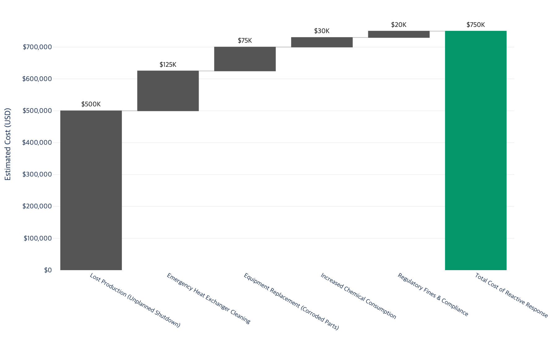
The waterfall chart above breaks down the cumulative cost of a single reactive failure event. Lost production dominates at USD 500,000, but secondary costs including emergency cleaning, parts replacement, increased chemical consumption, and compliance penalties accumulate to approximately USD 750,000 total. Proactive monitoring that catches degradation two to four weeks earlier typically costs less than 5 percent of this figure.

Why Standard Monitoring Misses Early Signals

Most facilities monitor pH, conductivity, and inhibitor residuals against fixed target ranges. As long as values fall within specification, the system is considered healthy. This approach has two fundamental flaws. First, it treats each parameter independently, missing the interactions between indicators that are far more predictive than any single value. Second, it focuses on whether the current reading is acceptable rather than whether the trend is moving toward failure.

A pH of 7.8 is within range for most phosphate-based treatment programs. But a pH that has drifted from 8.2 to 7.8 over three weeks tells a very different story. That 0.4-unit downward drift may indicate that the buffer capacity of the treatment program is being overwhelmed, possibly by increasing biological acid production or by a change in makeup water alkalinity. The trend, not the snapshot, is the early warning. Combining two or three mild indicator deviations is more predictive of impending failure than a single severe deviation (Water Technology Online, 2022).

The Hidden Cost of Late Detection

Beyond the direct financial impact of emergency shutdowns, late detection carries compounding costs that are often invisible in maintenance budgets. When fouling progresses past the point where chemical treatment can reverse it, mechanical cleaning becomes necessary. But mechanical cleaning itself introduces risks: tube damage during hydroblasting, gasket failures during reassembly, and shortened equipment service life from repeated cleaning cycles. A facility that cleans reactively four times per year instead of proactively once per year will see measurably shorter heat exchanger tube life, driving capital replacement costs that rarely get attributed to the original water treatment failure.

II. Five Leading Indicators and Their Degradation Mechanisms

Cooling water system degradation follows predictable patterns across five measurable parameters. Each indicator connects to a specific degradation mechanism, transforming raw data into actionable intelligence. Understanding the mechanism behind each indicator is what separates a number on a log sheet from a decision point.

Conductivity Drift

Conductivity measures total dissolved solids (TDS) and serves as the primary indicator of concentration cycles. In a properly controlled system, conductivity remains stable because blowdown removes concentrated water at the same rate evaporation concentrates it. When conductivity drifts upward, it signals that dissolved minerals are accumulating beyond design limits.

As conductivity rises, the Langelier Saturation Index (LSI) shifts positive, indicating supersaturation with calcium carbonate. The LSI is calculated from pH, temperature, calcium hardness, alkalinity, and TDS. An LSI above +0.5 indicates active scaling tendency, while values between -0.3 and +0.3 represent balanced conditions (Lenntech, 2023). Because LSI is influenced by multiple variables that all shift with rising TDS, a conductivity increase has a compounding effect on scale potential that is not immediately obvious from the conductivity reading alone.

A conductivity increase of 10 to 15 percent above setpoint sustained over 48 hours should trigger investigation. The most common root cause is a malfunctioning blowdown controller or valve. However, a conductivity rise can also result from a change in makeup water quality, process leaks introducing dissolved solids, or seasonal evaporation rate changes. Identifying the source determines the correct response. Simply increasing blowdown when the root cause is a process leak wastes water and treatment chemicals while failing to address the underlying problem.

pH Instability

Stable pH indicates chemical treatment equilibrium. When pH fluctuates beyond 0.3 units within 24 hours, the buffer capacity is being overwhelmed. The direction and pattern of the instability reveal the mechanism at work.

Downward drift accelerates corrosion, with rates approximately doubling for each full pH unit drop below 7.0 (Veolia Water Technologies, 2023). Sustained operation below pH 6.5 can cause rapid pitting on mild steel surfaces. Upward drift promotes calcium carbonate and calcium phosphate scale formation, particularly on heat transfer surfaces where local temperatures exceed bulk water temperatures.

The most concerning pattern is frequent oscillation. This often indicates biological acid production from sulfate-reducing bacteria (SRB) within biofilm layers. The oscillation occurs because biocide additions temporarily suppress acid production, but surviving bacteria resume activity as biocide residuals decay. This pattern signals simultaneous chemical and biological degradation. Operators who see oscillating pH and respond only with acid or caustic feed are treating the symptom while the root cause continues to advance.

Corrosion Coupon Trends

Corrosion coupons are sacrificial metal strips placed in the system for 90 to 120 days, then analyzed for weight loss to determine average corrosion rates (Tower Water, 2023). A single reading provides limited value because it represents an average over the entire exposure period. The real diagnostic power comes from tracking the trend across successive cycles.

A single reading of 2.0 mils per year (mpy) for mild steel may be acceptable. But a sequence showing 1.2, 1.5, 1.8, and 2.0 mpy over successive quarters indicates steadily declining protection, even though every individual reading falls within the "acceptable" range. The Association of Water Technologies (AWT) provides detailed standards: for carbon steel, rates below 1.0 mpy are good, 1.0 to 3.0 mpy indicate moderate conditions, and above 5.0 mpy requires immediate action (AWT, 2023). For copper alloys, the scale is much tighter: below 0.1 mpy is excellent, and anything above 0.5 mpy requires investigation (AWT, 2023).

Linear Polarization Resistance (LPR) devices offer near-real-time corrosion rate data, with measurements available within minutes rather than after a 90-day exposure period (ALSPI, 2023). LPR probes are particularly useful for detecting corrosion upsets and evaluating treatment adjustments in real time, though readings should be interpreted alongside coupon data rather than replacing it.

Biological Counts

Microbiological monitoring measures total viable organisms, reported as colony-forming units per milliliter (CFU/mL). Rising planktonic counts indicate that biofilm growth on system surfaces is exceeding biocide control. Planktonic counts represent only a fraction of the total microbial population. For every organism detected in a bulk water sample, there may be 100 to 1,000 times more organisms embedded in biofilm on pipe walls and heat exchanger surfaces.

Counts below 1,000 CFU/mL are considered controlled. Counts between 1,000 and 10,000 CFU/mL indicate declining biocide effectiveness. Above 10,000 CFU/mL represents significant growth requiring immediate intervention (Environmental Safety Technologies, 2023). The Cooling Tower Institute (CTI) recommends that total planktonic counts should not exceed 10,000 CFU/mL as an upper operational limit.

Uncontrolled biological growth also raises Legionella risk. ASHRAE Standard 188-2021 mandates water management plans for building water systems that create conditions conducive to Legionella growth (ASHRAE, 2021). The CDC estimates that 52,000 to 70,000 Americans suffer from Legionnaires' disease each year, with cooling towers identified as a significant transmission pathway (National Academies, 2019). Safe thresholds are below 10 CFU/mL for Legionella pneumophila serogroup 1 (CDC, 2023). The regulatory framework continues to tighten, making biological monitoring not only a performance issue but a compliance concern.

ATP (adenosine triphosphate) testing provides rapid biological assessment within minutes, offering a practical screening tool between formal heterotrophic plate count (HPC) analyses. A rising ATP trend reliably indicates increasing biological activity and should trigger more detailed investigation.

Heat Transfer Efficiency Decline

Heat transfer efficiency, measured through the approach temperature or overall heat transfer coefficient (U-value), is the most direct indicator of fouling. While the previous four indicators measure the conditions that lead to fouling, heat transfer efficiency measures fouling itself.

A 1 mm layer of calcium carbonate scale reduces efficiency by 10 to 12 percent, while the same thickness of biofilm reduces it by 15 to 20 percent due to the insulating properties of organic material (IntechOpen, 2022). More than 90 percent of heat transfer equipment is exposed to fouling formation during its operational life (IntechOpen, 2022). Reduced cooling capacity forces process units to derate, increasing energy consumption per unit of production.

A U-value decline exceeding 10 percent from the clean baseline indicates fouling requiring attention. Beyond 20 percent decline, mechanical cleaning is typically required. The approach temperature provides a simpler proxy for facilities that do not calculate U-values routinely. A rising approach temperature over successive days, with stable process-side conditions, indicates progressive fouling on the water side.

III. How Indicator Interactions Amplify Risk

The real predictive power comes from recognizing how indicators interact. Cooling water degradation follows cascade patterns where one form of degradation accelerates others. The chemistry, biology, and physics of a cooling water system are coupled, and failures in one domain accelerate failures in adjacent domains.

The Conductivity-pH-Scale Cascade

When conductivity rises from insufficient blowdown, increased mineral concentration shifts the LSI positive and raises pH through increased alkalinity. This dual effect creates conditions for rapid calcium carbonate scale formation. The relationship is nonlinear: a 20 percent increase in conductivity can shift the LSI from balanced (+0.2) to actively scaling (+0.8 or higher), because calcium hardness, alkalinity, and pH all shift together as concentration cycles increase.

Scale deposits create localized hot spots beneath the deposit layer. The metal surface temperature under a 1 mm scale layer can be 15 to 25 degrees Celsius higher than the bulk water temperature. These elevated temperatures further concentrate minerals in the thin water film beneath the deposit, accelerating growth in a positive feedback loop. The cascade extends to corrosion: the oxygen-depleted, chemically concentrated environment beneath scale deposits creates differential aeration cells that pit through tube walls far faster than general corrosion rates suggest.

The Biology-Corrosion Connection

Biofilm and corrosion are linked through microbiologically influenced corrosion (MIC). Sulfate-reducing bacteria within biofilms produce hydrogen sulfide that attacks steel surfaces directly. Iron-oxidizing bacteria create tubercles that establish differential aeration cells. Approximately 20 percent of all corrosion damage to metallic structures is attributed to microbial activity (ScienceDirect, 2023).

When biological counts rise simultaneously with increasing corrosion coupon rates, MIC should be suspected. This combination is more predictive of failure than either indicator alone. Standard biocide treatments that control planktonic bacteria may not penetrate established biofilm matrices, requiring targeted biodispersant programs to address the root cause. The biology-corrosion connection creates a self-sustaining cycle: corrosion products provide nutrients for iron-oxidizing bacteria, which accelerate further corrosion. Once established, MIC will not self-correct even if water chemistry returns to target ranges.

Figure 1. Single Severe Indicator vs Multiple Mild Indicators: Comparative Risk Profile

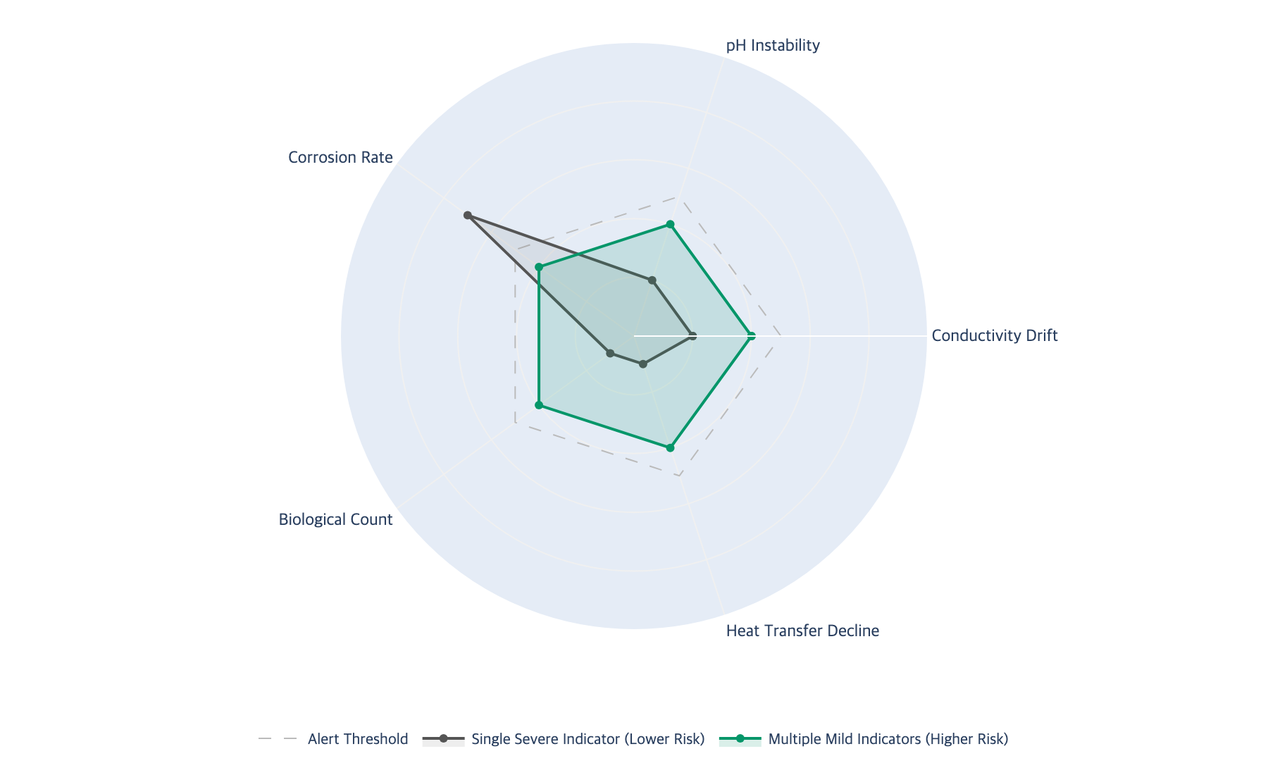
The radar chart above illustrates why multi-parameter monitoring outperforms single-variable tracking. A system with one indicator at critical level but four others normal appears less dangerous than a system with all five indicators at moderate deviation. Field experience confirms that the latter pattern is more predictive of imminent failure because it signals systemic degradation rather than an isolated upset.

Figure 2. Degradation Cascade: Trigger Conditions and Indicator Interactions

Trigger Condition	Primary Indicator	Secondary Indicator	Mechanism	Timeline
Blowdown controller malfunction	Conductivity rise >15%	pH drift upward	CaCO3 scale formation	2-4 weeks
Biocide underdosing	Biological count >10,000 CFU/mL	Heat transfer decline >10%	Biofilm + biofouling	1-3 weeks
Inhibitor feed pump failure	Corrosion coupon trend rising	pH instability	Accelerated corrosion	3-6 weeks
Makeup water quality change	Conductivity + pH shift together	LSI shift positive	Combined scale + corrosion	2-4 weeks
Seasonal temperature increase	Biological count rise	Conductivity rise	Bio-scale composite fouling	2-6 weeks

No single indicator tells the complete story. The combination of primary and secondary indicator deviations narrows the diagnosis and provides a more accurate timeline for intervention. Field engineers should look for the trigger conditions that match their facility's seasonal patterns and operational changes.

IV. Threshold Framework: Watch, Alert, and Critical Levels

A practical monitoring framework requires clear threshold levels calibrated to system type and metallurgy. Without defined action levels, operators are forced to make judgment calls on each data point, introducing inconsistency and delay. The following defines three action levels for each indicator, applicable to open recirculating systems with mild steel metallurgy and phosphate-based inhibitor programs.

Figure 3. Traffic-Light Threshold Summary by Indicator and Action Level

Indicator	Watch	Alert	Critical	Response Timeline
Conductivity (% above setpoint)	10-15% for >24h	15-20% for >48h	>20%	Verify within 4h
pH (deviation from target)	>0.3 units for >12h	>0.5 units	>1.0 unit	Inspect within 2h
Corrosion Rate, mild steel (mpy)	2.0-3.0, rising trend	3.0-5.0	>5.0	Next coupon cycle or immediate LPR
Biological Count (CFU/mL)	1,000-5,000	5,000-10,000	>10,000	Adjust biocide within 24h
Heat Transfer U-value (% decline)	5-10% from baseline	10-20%	>20%	Schedule cleaning within 1 week

Each threshold level triggers a specific, predefined response. Watch means increased monitoring frequency and root cause investigation. Alert requires corrective action within the specified timeline and notification of the responsible engineer. Critical demands immediate intervention, with production operations notified of potential shutdown risk.

Calibrating Thresholds to Your System

This framework should be calibrated to site-specific conditions. Systems with copper alloy metallurgy require significantly tighter corrosion thresholds, with Watch beginning at 0.25 mpy and Critical at 0.5 mpy. High-temperature climates may need adjusted biological thresholds due to accelerated microbial growth. Systems operating at higher concentration cycles will have tighter conductivity thresholds because the margin between normal operation and scaling conditions is narrower.

Facilities with multiple cooling loops should establish separate threshold sets for each loop. A cooling water system serving a reactor with 300-degree Celsius process temperatures operates under fundamentally different fouling risk than one serving an ambient-temperature storage tank. The key principle is that each threshold level triggers a defined response action, eliminating ambiguity.

The Role of ORP in Threshold Monitoring

Oxidation-reduction potential (ORP) provides a complementary measurement that strengthens the threshold framework, particularly for biological control. ORP values in cooling towers should be maintained in the range of 650 to 750 millivolts for effective microbial control (ChemREADY, 2024). A declining ORP trend, even when biological counts have not yet risen, can signal that biocide residuals are being consumed faster than they are being applied. This makes ORP a leading indicator for biological upsets, providing warning before planktonic counts confirm the problem.

V. From Data Patterns to Maintenance Decisions

Real-world decisions require interpreting indicator combinations rather than reacting to individual values. Conductivity rising with upward pH drift indicates scaling conditions, requiring immediate blowdown correction. If conductivity rises with stable pH, a process leak introducing dissolved solids is more likely, requiring a different investigation path.

Biological counts rising with declining heat transfer confirms biofouling. When this pattern appears, assess whether biofilm has established to the point where it protects organisms from biocide contact. A biodispersant program may be needed before biocide additions can reach organisms within the biofilm matrix.

Corrosion rates increasing with pH instability suggests inhibitor disruption, requiring pH stabilization first. Increasing the inhibitor dose without stabilizing pH is ineffective because phosphate-based inhibitors require a minimum pH to form protective films. Below pH 7.0, most phosphate inhibitors lose effectiveness regardless of dose.

The most critical pattern is multiple indicators at watch level simultaneously. When three or more indicators enter the watch zone, the system is approaching a tipping point even though no single parameter has reached alert level. The appropriate response is to treat it as an alert-level event.

When to Adjust Treatment Versus Shut Down for Cleaning

If indicators respond to treatment adjustments within one to two weeks, the degradation is in early stages and chemical control is sufficient. Watch for conductivity returning to within 5 percent of setpoint, pH stabilizing within target range, and biological counts trending downward. These responses confirm reversible fouling.

If indicators do not respond within two weeks, or if heat transfer efficiency has declined beyond 20 percent, physical cleaning is required. Delaying the shutdown decision typically results in higher cleaning costs, longer downtime, and risk of permanent tube damage from under-deposit corrosion.

Seasonal Monitoring Adjustments

Summer months bring elevated water temperatures that accelerate both biological growth and scaling tendency. Every 10-degree Celsius increase approximately doubles biological growth rates and shifts the LSI toward more positive values. During peak summer, biological monitoring frequency should increase from weekly to twice weekly, and conductivity setpoints may need to be lowered. During winter or reduced-load periods, the focus shifts to corrosion monitoring in low-flow areas where stagnant zones accelerate localized corrosion.

Monitoring Frequency Recommendations

Under normal conditions, conductivity, pH, and ORP should be monitored continuously with hourly logging. Biological counts should be measured weekly using ATP testing, supplemented by monthly HPC analysis. Corrosion coupons should be analyzed on 90-day cycles, with LPR devices providing real-time data where justified (ALSPI, 2023). Heat transfer efficiency should be calculated daily from logged process data. When any indicator enters the alert zone, all parameters should be monitored at maximum frequency until resolved.

Bridging the Data Silo

In many facilities, water treatment data and process operations data exist in separate systems managed by different teams. The water treatment operator monitors chemistry while the process engineer monitors heat exchanger performance. Neither team routinely reviews the other's data. Heat transfer efficiency decline is the earliest physical signal of fouling, but it is often visible only in process data systems that the water treatment team does not access. A weekly cross-functional review where water treatment trends are overlaid with heat exchanger performance data is sufficient to identify multi-parameter patterns that neither team would catch independently.

VI. Key Takeaway

• Monitor trends, not snapshots. A parameter moving toward failure is more important than a parameter already out of range. A rising trend still within specification is an early warning; an out-of-range reading is a late alarm.

• Combine indicators for prediction. Two or three mild deviations occurring simultaneously are more predictive of impending failure than a single severe deviation.

• Calibrate thresholds to your system. The watch-alert-critical framework must be adjusted for your specific metallurgy, operating temperatures, concentration cycles, and seasonal conditions.

• Integrate water treatment and process data. Heat transfer efficiency decline is the earliest physical signal of fouling, but it is often siloed in process operations.

• Act on watch-level combinations. When multiple indicators enter the watch zone simultaneously, treat it as an alert-level event and initiate a comprehensive system review.

Lubinpla's AI-powered diagnostic assistant can cross-reference cooling water monitoring data across all five leading indicators simultaneously, identifying multi-parameter degradation patterns that single-variable programs miss. By analyzing trend direction, rate of change, and indicator interactions against your system's specific metallurgy and operating conditions, Lubinpla recommends treatment adjustments before degradation cascades reach the point where chemical intervention alone is no longer sufficient.

VII. References

[1] NACE International, "Cost of Corrosion Study", 2023. https://www.nace.org/resources/general-resources/corrosion-basics

[2] Water Technology Online, "Cooling Water Control and Online Corrosion Monitoring", 2022. https://www.watertechonline.com/home/article/14171015/cooling-water-control-and-online-corrosion-monitoring

[3] Veolia Water Technologies, "Cooling Water Corrosion Control Handbook", 2023. https://www.watertechnologies.com/handbook/chapter-24-corrosion-control-cooling-systems

[4] Veolia Water Technologies, "Monitoring and Control of Water Treatment Handbook", 2023. https://www.watertechnologies.com/handbook/chapter-36-monitoring-and-control-water-treatment

[5] Tower Water, "Corrosion Coupon Rack Monitoring for Cooling Tower Systems", 2023. https://towerwater.com/corrosion-coupon-rack-cooling-tower-monitoring/

[6] Lenntech, "Langelier Saturation Index Calculator", 2023. https://www.lenntech.com/calculators/langelier/index/langelier.htm

[7] CDC, "Controlling Legionella in Cooling Towers", 2023. https://www.cdc.gov/control-legionella/php/toolkit/cooling-towers-module.html

[8] Environmental Safety Technologies, "Cooling Tower Legionella and Microbiological Tests", 2023. https://estechlab.com/cooling-tower-legionella-microbiological-tests/

[9] IntechOpen, "Fouling in Industrial Heat Exchangers: Formation, Detection and Mitigation", 2022. https://www.intechopen.com/chapters/82043

[10] M4 Knick, "Cooling Tower Corrosion Monitoring: pH, ORP and Conductivity", 2023. https://m4knick.com/cooling-tower-corrosion-monitoring/

[11] SAMCO Technologies, "Treated vs. Untreated Cooling Tower Water: Risks for Your Plant", 2023. https://samcotech.com/treated-vs-untreated-cooling-tower-water-risks-problems/

[12] AWT, "Standards for Corrosion Rates", 2023. https://bondwater.com/docs/techpapers/corrosion_rates.pdf

[13] ALSPI, "Introduction to Linear Polarization Resistance (LPR) Monitoring", 2023. https://www.alspi.com/lprintro.htm

[14] ScienceDirect, "Microbiologically Influenced Corrosion of Circulating Cooling Systems in Power Plants", 2023. https://www.sciencedirect.com/science/article/pii/S1878535223009917

[15] ASHRAE, "ANSI/ASHRAE Standard 188-2021: Legionellosis Risk Management for Building Water Systems", 2021. https://www.ashrae.org/technical-resources/bookstore/ansi-ashrae-standard-188-2021-legionellosis-risk-management-for-building-water-systems

[16] ChemREADY, "Understanding ORP in Cooling Towers: Importance, Monitoring, and Best Practices", 2024. https://www.getchemready.com/water-facts/understanding-orp-in-cooling-towers-importance-monitoring-and-best-practices/

[17] National Academies of Sciences, Engineering, and Medicine, "Management of Legionella in Water Systems", 2019. https://nap.nationalacademies.org/catalog/25474/management-of-legionella-in-water-systems

---

Powered by Lubinpla

Discover how technical teams solve complex challenges faster with AI.

Learn More About Lubinpla