How Small Dosage Adjustments in Water Treatment Cut Chemical Costs by 20%

Summary: Most industrial water treatment programs operate with chemical dosages 15 to 30 percent above the minimum effective concentration, built on worst-case safety margins rather than actual operating data. This article explains the diminishing returns relationship between inhibitor concentration and protection effectiveness, presents a data-driven methodology for finding the optimal dosing zone, and provides a step-down protocol with defined safety checkpoints for reducing chemical spend by 15 to 25 percent while maintaining or improving system protection. It also examines the monitoring technologies that make real-time dosage optimization practical and introduces a field case study demonstrating the full optimization cycle from baseline assessment through validated cost reduction.

Table of Contents

I. Why Most Water Treatment Programs Are Overdosed

II. The Diminishing Returns Curve: Concentration vs Protection

III. Data-Driven Dosage Optimization Methodology

IV. The Step-Down Protocol: Reducing Dosage Safely

V. Monitoring Technologies That Enable Optimization

VI. Field Case: Cooling Tower Inhibitor Optimization

VII. Validation and Monitoring Framework

VIII. Key Takeaway

IX. References

I. Why Most Water Treatment Programs Are Overdosed

A water treatment program designed for a cooling tower system typically specifies inhibitor concentrations based on the most aggressive conditions the system could encounter: peak summer temperatures, maximum concentration cycles, worst-case makeup water quality, and lowest flow rates. These design conditions may occur for a few weeks per year, but the dosage is maintained year-round. The result is a program that delivers significantly more chemical than needed during the majority of operating hours.

The financial impact is meaningful. Chemical costs represent 15 to 25 percent of total water treatment operational expenses for a typical industrial facility, with inhibitor chemicals accounting for the largest share (PORVOO, 2024). A facility spending USD 200,000 annually on water treatment chemicals that is overdosing by 20 percent is spending approximately USD 40,000 per year on chemicals that provide no additional protection. Over a five-year period, that excess accumulates to USD 200,000, the equivalent of a major system upgrade or a full year of treatment at the optimized rate.

How Safety Margins Compound Over Time

The overdosing problem is compounded by multiple layers of safety margins. The chemical supplier recommends a concentration range with a built-in safety factor. The site water treatment specialist adds a margin above the supplier recommendation to account for upset conditions. The control system is set to alarm at the lower end of this already-elevated range, so operators maintain dosage well above the alarm point. Each layer of margin is individually rational, but the cumulative effect is a program running 15 to 30 percent above the true minimum effective concentration.

Consider a typical phosphate-based corrosion inhibitor program. The supplier specifies a target range of 15 to 25 ppm orthophosphate as PO4. The site specialist, aware that summer peak loads push the system harder, sets the operating target at 22 to 25 ppm. The control system alarms at 18 ppm, well below the operating target but also well above the minimum effective concentration. Operators, trained to avoid alarms, keep the residual at 24 to 28 ppm. What started as a 15 to 25 ppm range effectively becomes a 24 to 28 ppm operating reality, nearly double the minimum effective concentration for most of the year.

The Overlooked Cost of Overdosing

Beyond direct chemical costs, overdosing creates secondary expenses that are often invisible in the treatment budget. Higher inhibitor concentrations increase blowdown water treatment costs because more dissolved solids must be removed from the system. Excess phosphate-based inhibitors can contribute to biological growth by providing nutrients to microorganisms. In fact, phosphorus is the limiting nutrient for algae growth in most water systems, meaning that every additional ppm of orthophosphate above the effective minimum directly fuels biological fouling. Research has shown that 1 pound of excess phosphorus can produce up to 500 pounds of wet algae in the receiving environment (Veolia, 2023). This excess biological load then requires additional biocide treatments, creating a cascading cost increase.

In some cases, overdosing corrosion inhibitors beyond the optimum level can actually reduce effectiveness, as research has shown that increasing inhibitor dosage beyond the optimal concentration may have a detrimental effect on corrosion protection (SUT, 2023). When orthophosphate concentrations exceed approximately 10 ppm at elevated temperatures and pH levels above 7.5, the risk of tricalcium phosphate (Ca3(PO4)2) scaling increases significantly (Water Technology Report, 2018). This calcium phosphate scale deposits preferentially on the hottest heat transfer surfaces, reducing thermal efficiency and potentially causing localized under-deposit corrosion, the very failure mode the inhibitor was meant to prevent.

The Hidden Energy Penalty

There is also an energy cost to overdosing that rarely appears in treatment program evaluations. Scale deposits as thin as 0.5 mm on heat exchanger surfaces can reduce heat transfer efficiency by 10 to 15 percent. When phosphate overdosing contributes to calcium phosphate fouling on condenser tubes or heat exchanger surfaces, the facility compensates by running cooling equipment harder or longer. Corrosion inhibitors, when properly dosed, improve heat transfer and can reduce energy consumption by up to 30 percent in cooling systems (Gradiant, 2023). Paradoxically, overdosing the same inhibitor can reverse this benefit by creating the fouling conditions that degrade heat transfer.

II. The Diminishing Returns Curve: Concentration vs Protection

The relationship between inhibitor concentration and corrosion protection is not linear. At very low concentrations, protection effectiveness increases steeply with each increment of added chemical. As concentration increases, each additional increment provides less additional protection until a plateau is reached where further increases yield negligible benefit. Understanding this curve is the foundation of every successful dosage optimization effort.

Understanding the Optimal Dosing Zone

The optimal dosing zone exists at the point where the protection curve begins to flatten, where the last meaningful increment of protection is achieved before diminishing returns dominate. Below this zone, the system is under-protected and corrosion rates will increase unacceptably. Above this zone, additional chemical provides no measurable improvement in protection while increasing costs.

For phosphate-based corrosion inhibitors in cooling water systems, the protection curve typically shows 80 to 85 percent of maximum effectiveness at 50 to 60 percent of the commonly specified concentration. The remaining 15 to 20 percent of effectiveness requires the other 40 to 50 percent of chemical. This mathematical reality means that modest reductions from the over-dosed state, perhaps 15 to 25 percent, can be achieved while remaining well within the effective zone of the protection curve.

The shape of this curve is governed by adsorption thermodynamics. Corrosion inhibitors work by adsorbing onto the metal surface to form a protective barrier. At low concentrations, there are abundant available surface sites, so each additional molecule of inhibitor finds an open site and contributes to protection. As coverage increases, fewer open sites remain, and each additional molecule must compete for remaining positions. Beyond a certain coverage threshold, typically 85 to 95 percent surface coverage, additional inhibitor molecules have virtually no available sites and remain in solution without contributing to protection.

Figure 1. The Diminishing Returns Curve: Inhibitor Concentration vs Protection Effectiveness

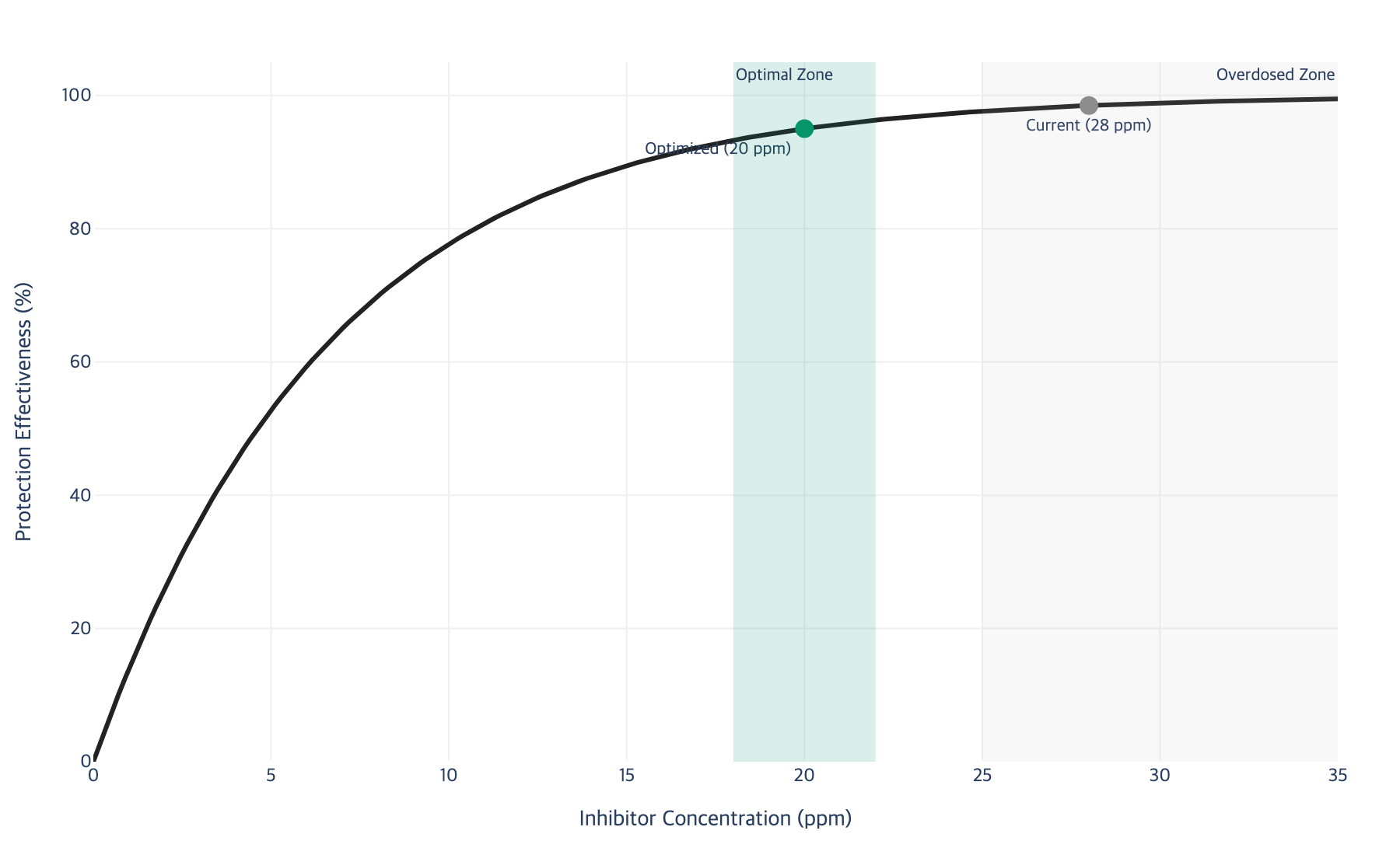
The curve above illustrates why modest dosage reductions have minimal impact on protection. Moving from the typical overdosed point (28 ppm) to the optimized target (20 ppm) represents a 28 percent chemical reduction while remaining on the plateau portion of the curve where protection is near-maximum. The green zone identifies the optimal dosing range where maximum protection is achieved with minimum chemical consumption. The steep region below 12 ppm shows where protection drops rapidly and dosage reductions become dangerous. The flat region above 22 ppm is where most overdosed programs operate, spending heavily for negligible additional protection.

Why the Minimum Effective Concentration Varies

The minimum effective concentration is not a fixed number; it varies with system conditions. Water temperature, pH, total dissolved solids, flow velocity, and metallurgy all influence the concentration required for adequate protection. This is precisely why worst-case design margins exist, to cover the full range of operating conditions with a single dosage setpoint. The opportunity for optimization lies in adjusting dosage in response to actual conditions rather than maintaining a fixed setpoint designed for worst-case conditions.

Temperature is the most significant variable. As water temperature increases, corrosion reaction kinetics accelerate, and the minimum inhibitor concentration required for adequate surface coverage rises. A system that achieves full protection at 16 ppm during winter months (inlet water at 15 degrees C) may require 22 ppm during peak summer (inlet water at 32 degrees C). If the program is designed for the summer peak and maintained year-round, the system is overdosed by approximately 37 percent during colder months.

Cycles of concentration introduce another variable. Increasing cycles from three to six reduces cooling tower makeup water by 20 percent and blowdown by 50 percent, but it also concentrates all dissolved solids, including inhibitors, in the recirculating water (US DOE, 2023). When cycles increase seasonally, the effective inhibitor concentration in the recirculating water may already exceed the target without any increase in chemical feed rate. Programs that do not account for this concentration effect are overdosing by the same factor as the cycle increase.

III. Data-Driven Dosage Optimization Methodology

Optimization requires replacing assumption-based dosing with data-driven dosing. The methodology follows four phases: baseline assessment, correlation analysis, target identification, and controlled adjustment. Each phase builds on the findings of the previous one, and no phase should be skipped or shortened.

Phase 1: Baseline Assessment (4 to 8 Weeks)

Before adjusting any dosage, establish a quantitative baseline of current system performance. Record the following parameters at increased frequency (daily or continuous where possible): inhibitor residual concentration, corrosion rates (coupon data and/or LPR), system water chemistry (pH, conductivity, alkalinity, hardness), process conditions (temperatures, flow rates, heat loads), and chemical consumption volumes.

This baseline serves two purposes. It documents the current level of over-protection, which quantifies the optimization opportunity. It also establishes the performance metrics that must be maintained during and after dosage adjustment. Without a rigorous baseline, there is no objective way to determine whether a subsequent dosage reduction has compromised protection or simply removed unnecessary excess.

The baseline period should span at least one full operating cycle that includes both normal and elevated demand conditions. For facilities with strong seasonal variation, consider extending the baseline to capture the transition from mild to peak conditions. This ensures that the correlation analysis in Phase 2 includes data points across the range of conditions the system will encounter.

Phase 2: Correlation Analysis

Analyze the baseline data to identify the relationship between inhibitor concentration and corrosion performance under your actual operating conditions. The key question is: at what inhibitor concentration does corrosion rate begin to increase measurably? If the current inhibitor residual runs at 25 ppm and corrosion rates are consistently below 1.5 mpy, the effective concentration may be closer to 18 to 20 ppm. The correlation between residual concentration and corrosion rate reveals the shape of the diminishing returns curve for your specific system.

Plot the inhibitor residual concentration on the x-axis against the corresponding corrosion rate on the y-axis for every data point in the baseline period. If the system is significantly overdosed, the scatter plot will show a cluster of data points on the flat plateau region of the curve, with corrosion rates remaining essentially constant across a wide range of inhibitor concentrations. This plateau is the quantitative evidence of overdosing. The lower boundary of this plateau, where corrosion rate begins to rise with decreasing concentration, marks the beginning of the minimum effective concentration zone.

Include operating conditions as covariates in the analysis. A single concentration-versus-corrosion plot may show apparent scatter that resolves into distinct curves when stratified by temperature range or cycle of concentration. For instance, data points collected during summer months may show a higher minimum effective concentration than winter data points. This stratification reveals the seasonal adjustment factors needed for an optimized program.

Phase 3: Target Identification

Based on the correlation analysis, identify a target concentration that maintains the corrosion rate below the acceptable threshold while reducing chemical usage. The target should include a 10 to 15 percent margin above the minimum effective concentration to provide a safety buffer without the excessive margins of the original program. For example, if analysis shows that corrosion rates remain below 2.0 mpy at 18 ppm and begin to rise at 15 ppm, a target of 20 ppm provides adequate protection with margin while reducing from the current 25 ppm dosage, a 20 percent reduction.

The acceptable corrosion rate threshold varies by system metallurgy and operating requirements. For mild steel systems, 2.0 to 3.0 mpy is generally acceptable for cooling water service. For copper alloy condenser tubes, the threshold is lower, typically below 0.5 mpy. Define these thresholds before beginning the target identification process so that the optimization has a clear, objective success criterion.

Phase 4: Controlled Adjustment

Implement the dosage reduction gradually using the step-down protocol described in the next section. Never reduce dosage in a single step to the target concentration. Gradual reduction allows the system to equilibrate at each level and provides early warning if the reduction is approaching the effective limit. Abrupt reductions risk destabilizing the protective film on metal surfaces, potentially causing a transient corrosion spike even if the new steady-state concentration would be adequate.

IV. The Step-Down Protocol: Reducing Dosage Safely

The step-down protocol provides a structured approach to reducing chemical dosage while continuously monitoring system health. Each step reduces concentration by a defined increment, holds for a defined period, and evaluates against defined reversal triggers before proceeding to the next step. This structured approach removes guesswork and provides objective decision criteria at every stage.

Protocol Structure

Step 1: Reduce inhibitor feed rate by 5 percent from baseline. Hold for two weeks. Monitor corrosion rate, inhibitor residual, and system chemistry daily. If all parameters remain within acceptable limits, proceed to Step 2. Step 2: Reduce by an additional 5 percent (10 percent total reduction). Hold for two weeks with the same monitoring. Step 3: Reduce by another 5 percent (15 percent total). Hold for three weeks because the margin above minimum effective concentration is now thinner. Step 4: If the target reduction is 20 percent or more, reduce by the final increment. Hold for four weeks with intensified monitoring.

The hold periods are not arbitrary. The two-week hold at Steps 1 and 2 allows sufficient time for the system to reach a new equilibrium. When inhibitor concentration is reduced, the existing protective film on metal surfaces gradually thins as molecules desorb and are not fully replaced. This thinning process takes several days to stabilize. The longer hold periods at Steps 3 and 4 reflect the fact that the protective film is now thinner and the system is operating closer to the minimum effective concentration, where small variations in water chemistry or operating conditions could have a larger impact on corrosion rates.

Defined Reversal Triggers

At any step, immediately reverse to the previous concentration level if corrosion rates increase by more than 30 percent from baseline, if inhibitor residual drops below the minimum level identified in Phase 2, if system upset conditions occur (pH excursion, conductivity spike, temperature increase), or if biological counts increase by more than one order of magnitude. A reversal is not a failure of the optimization. It is the protocol working as designed, identifying the actual boundary of the optimal dosing zone.

When a reversal is triggered, document the conditions that caused the trigger, the concentration level at which it occurred, and the time elapsed since the last step-down. This information refines the correlation analysis and helps define the true minimum effective concentration under the specific conditions that caused the trigger. After conditions stabilize and the reversal trigger clears, the step-down can be resumed if the trigger was caused by a transient condition rather than a fundamental dosage limitation.

Seasonal Adjustment Protocol

Recognize that the minimum effective concentration varies seasonally. The optimized dosage identified during mild conditions may be insufficient during peak summer temperatures or periods of maximum process load. Build seasonal adjustment factors into the optimized program: higher dosage during high-demand months, lower dosage during mild months. This dynamic approach can achieve overall annual savings of 20 to 25 percent compared to the fixed worst-case dosage.

Seasonal variation in source water chemistry also affects the optimized dosage. Makeup water quality can change significantly between seasons, with spring runoff bringing higher turbidity and dissolved organics, while late summer may bring higher mineral content due to reduced reservoir levels. Conductivity-based blowdown control helps manage cycles of concentration automatically, but the inhibitor feed rate may still require seasonal adjustment to account for changes in makeup water composition and system demand. By making small adjustments early in the seasonal transition, operators avoid large swings in concentration and the corrosion rate spikes that can accompany sudden program changes (US DOE, 2023).

V. Monitoring Technologies That Enable Optimization

Dosage optimization depends entirely on the quality and frequency of monitoring data. The methodology described above requires near-real-time visibility into corrosion rates, inhibitor residuals, and water chemistry. Traditional monitoring approaches, which rely on periodic grab samples and quarterly coupon pulls, do not provide the data resolution needed for effective optimization.

Corrosion Monitoring: Coupons vs LPR Probes

Corrosion coupons have been the industry standard for decades. Metal test specimens are exposed to the system water for 90 to 100 days, then removed, cleaned, and weighed to determine average corrosion rate over the exposure period (Solenis, 2023). This method is reliable for establishing long-term trends but has a critical limitation for optimization work: it provides only an average rate over the entire exposure period. If a two-week dosage step-down causes a temporary corrosion spike that is followed by six weeks of normal performance, the coupon data will show a slightly elevated average with no indication of when the spike occurred or how severe it was.

Linear Polarization Resistance (LPR) probes address this limitation by providing instantaneous, real-time corrosion rate measurements. LPR probes measure the current response to a small applied voltage, yielding corrosion rate data on a daily or even hourly basis with resolution as fine as 0.001 mpy (Pyxis Lab, 2023). This real-time capability is essential for the step-down protocol because it allows operators to detect corrosion rate increases within hours of a dosage reduction, rather than waiting months for the next coupon pull.

The recommended approach is to use both methods simultaneously. LPR probes provide the real-time feedback needed for active optimization, while coupons provide the long-term validation and visual surface inspection that confirms the LPR data. If an upset occurs for a short period, the average corrosion rate measured by coupons may not change dramatically, making it very hard or even impossible to detect the upset with coupons alone (Solenis, 2023). The LPR probe will capture the event and trigger the reversal protocol before cumulative damage accumulates.

Online Chemistry Analyzers

Beyond corrosion monitoring, online analyzers for pH, conductivity, and inhibitor residual provide the continuous data streams that make adaptive dosing possible. Conductivity-based blowdown controllers maintain consistent cycles of concentration, preventing the concentration spikes that can cause scaling or the dilution events that can leave the system temporarily under-protected. Online phosphate analyzers track inhibitor residual in real time, enabling feed rate adjustments in response to changing demand rather than relying on a fixed feed rate calibrated to worst-case conditions.

The investment in monitoring equipment is modest relative to the savings it enables. A typical LPR probe system costs USD 2,000 to 5,000. Online chemistry analyzers range from USD 3,000 to 8,000 depending on the parameters measured. For a program spending USD 200,000 annually on chemicals, the monitoring investment represents 2 to 5 percent of one year's savings, with payback typically occurring within the first two to three months of optimized operation.

VI. Field Case: Cooling Tower Inhibitor Optimization

The following case study illustrates the complete optimization methodology applied to a multi-cell cooling tower system at an industrial manufacturing facility. The facility is anonymized, but the technical details and quantitative results are structurally representative of documented optimization outcomes.

Site Background

Company A operates a four-cell cooling tower system serving process heat exchangers and HVAC condensers at a manufacturing plant with year-round operation. The system circulates approximately 15,000 gallons per minute with a design heat rejection capacity of 4,500 tons. Makeup water is municipal supply with moderate hardness (180 ppm as CaCO3) and alkalinity (120 ppm as CaCO3). System metallurgy includes mild steel piping, copper alloy condenser tubes, and stainless steel heat exchanger plates. Annual water treatment chemical spend was approximately USD 210,000, of which USD 135,000 was phosphate-based corrosion and scale inhibitor.

The existing treatment program specified an orthophosphate residual target of 22 to 28 ppm at 4.5 to 5.5 cycles of concentration. The program had been unchanged for seven years, originally designed by the chemical supplier for the highest anticipated summer load conditions. Corrosion coupons pulled quarterly consistently showed mild steel corrosion rates between 0.8 and 1.4 mpy, well below the 3.0 mpy threshold.

Baseline Assessment Findings

A six-week baseline assessment with LPR probes and daily chemistry sampling revealed that the actual operating inhibitor residual averaged 26.3 ppm, near the top of the specified range. Corrosion rates measured by LPR averaged 1.1 mpy on mild steel and 0.12 mpy on copper alloy, both well below action thresholds. Water temperature during the baseline period ranged from 22 to 34 degrees C, and cycles of concentration ranged from 4.2 to 5.8.

The correlation analysis showed that corrosion rate remained below 1.5 mpy at all LPR data points where the orthophosphate residual was above 17 ppm. Below 17 ppm, which occurred briefly during two makeup water upsets, corrosion rates increased to 2.1 and 2.4 mpy before recovering when the residual returned to normal levels. This established 17 ppm as the approximate minimum effective concentration under the conditions observed during the baseline period.

Step-Down Execution

With a baseline average of 26.3 ppm and a minimum effective concentration of 17 ppm, the optimization target was set at 19.5 ppm (17 ppm plus a 15 percent margin). This represented a 26 percent reduction from the operating average. The step-down proceeded as follows. Step 1 reduced the feed rate to achieve a 21 to 24 ppm residual (approximately 8 percent reduction). After two weeks, corrosion rates remained at 1.1 mpy average. Step 2 reduced to 19 to 22 ppm residual (approximately 18 percent reduction). After two weeks, corrosion rates averaged 1.2 mpy with no upward trend. Step 3 reduced to 18 to 21 ppm residual (approximately 24 percent reduction). During the three-week hold, a two-day heat wave pushed water temperatures above 36 degrees C, and corrosion rates briefly increased to 1.8 mpy. The rate returned to 1.3 mpy as temperatures normalized. This was within acceptable limits, so the step-down continued. Step 4 held at the 18 to 21 ppm range through a four-week validation period that included both mild and warm weather. Corrosion rates averaged 1.25 mpy, confirming that the optimized dosage provided adequate protection.

Quantitative Results

The optimized program reduced the average orthophosphate residual from 26.3 ppm to 19.8 ppm, a 25 percent reduction. Annualized inhibitor chemical savings were USD 33,750 (25 percent of the USD 135,000 inhibitor spend). Additional savings of USD 4,200 came from reduced blowdown treatment costs due to lower phosphate loading in the blowdown stream. Biocide consumption decreased by approximately 8 percent (USD 2,100 annually) as the lower phosphate residual reduced nutrient availability for biological growth. Total annual savings reached USD 40,050. The monitoring equipment investment (two LPR probes, online phosphate analyzer, and data logging system) totaled USD 11,500, yielding a payback period of 3.4 months.

Corrosion performance at the optimized dosage (average 1.25 mpy on mild steel, 0.14 mpy on copper alloy) remained well within acceptable limits and showed no degradation over the subsequent twelve months of operation. The optimized program incorporated a seasonal adjustment factor that increased the target residual to 22 ppm during June through September and reduced it to 17 ppm during November through March, further improving the annual average savings compared to a single fixed target.

VII. Validation and Monitoring Framework

Dosage optimization is not a one-time project but an ongoing management approach. The optimized program requires sustained monitoring to confirm that protection levels remain adequate as conditions change. System modifications, changes in makeup water quality, new heat loads, or equipment additions can all shift the minimum effective concentration, requiring periodic re-evaluation of the optimized dosage target.

Figure 1. Dosage Optimization Step-Down Protocol and Monitoring Schedule

Phase	Duration	Dosage Change	Monitoring Frequency	Reversal Trigger
Baseline	4-8 weeks	None (establish baseline)	Daily: all parameters	Not applicable
Step 1	2 weeks	-5% from baseline	Daily: corrosion rate, residual, chemistry	Corrosion >30% above baseline
Step 2	2 weeks	-10% total	Daily: all parameters	Corrosion >30% above baseline
Step 3	3 weeks	-15% total	Daily: corrosion, residual; weekly: biology	Corrosion >30% or biology >10x baseline
Step 4	4 weeks	-20% total (if target)	Daily: all parameters	Any reversal trigger
Validation	8-12 weeks	Hold at optimized level	Weekly: standard program	Any sustained deviation
Ongoing	Continuous	Seasonal adjustments	Monthly: standard; daily during peak	Seasonal triggers

This schedule provides a clear roadmap for the entire optimization process, from baseline through ongoing management. The gradually increasing hold periods at each step reflect the decreasing safety margin as the dosage approaches the minimum effective concentration. The validation phase is particularly important because it extends through a complete seasonal cycle, confirming that the optimized dosage remains adequate under all operating conditions the system will encounter.

Figure 2. Annual Cost Savings Breakdown: From Current to Optimized Program

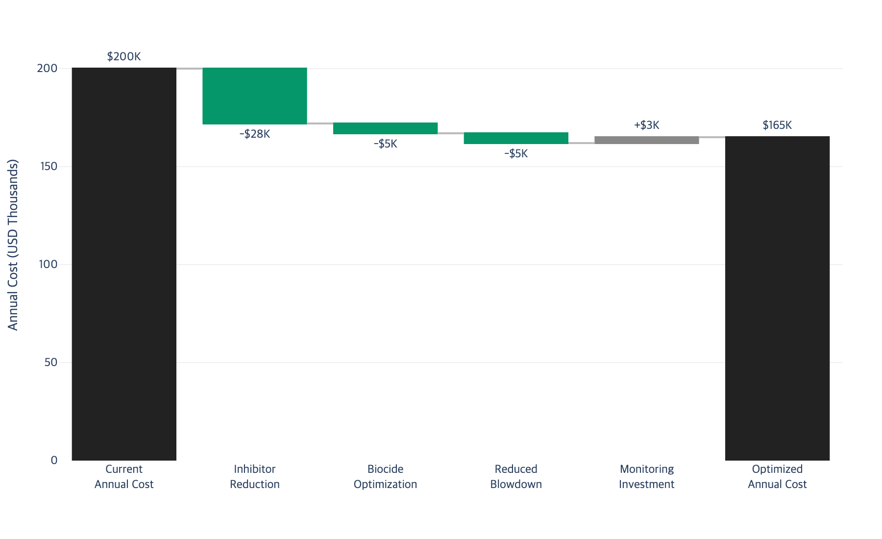
The waterfall chart above shows how a USD 200,000 annual chemical program can be reduced to approximately USD 165,000 through systematic optimization. Inhibitor reduction contributes the largest savings at USD 28,000, followed by biocide optimization and reduced blowdown costs. The monitoring equipment investment of USD 3,000 is a small fraction of the total savings, confirming the strong return on investment for data-driven optimization.

Key Performance Indicators for Ongoing Validation

Track three primary KPIs to confirm the optimized program is performing adequately over time. First, corrosion rate should remain below the site-specific target (typically 2.0 to 3.0 mpy for mild steel, below 0.5 mpy for copper alloys). Second, chemical cost per unit of treated water should show a measurable decrease from the pre-optimization baseline. Third, system cleanliness metrics (biological counts, heat transfer efficiency, scale deposition rates) should remain stable or improve.

Establish a monthly review cycle for these KPIs during the first year of optimized operation. If all three indicators remain within acceptable ranges for twelve consecutive months, the review frequency can be reduced to quarterly. Any single KPI deviation that persists for more than two weeks should trigger a return to daily monitoring and a review of whether system conditions have changed enough to warrant adjusting the optimized dosage target.

Documentation and Communication

Document the optimization process thoroughly, including baseline data, correlation analysis results, each step-down decision and outcome, and the final optimized parameters. This documentation is essential for justifying the program to management, training new operators, and re-baselining after system changes.

The documentation also serves as institutional knowledge preservation. When the water treatment specialist who conducted the optimization moves to another role or leaves the facility, the documented protocol and data allow a successor to understand why the program operates at its current dosage rather than the higher legacy specification. Without this documentation, the natural tendency is for a new specialist to revert to the manufacturer's recommended range, undoing the optimization and reintroducing the cost penalty.

Common Pitfalls in Long-Term Program Maintenance

Three common pitfalls undermine optimized programs over time. The first is alarm creep. Operators who are accustomed to the pre-optimization residual levels may view the optimized lower residual as a problem and gradually increase the feed rate back toward the original levels. Prevent this by updating alarm setpoints to reflect the optimized range and conducting operator training that explains the data supporting the new targets. The second pitfall is seasonal revert, where the temporary increase in dosage during peak summer months becomes the new year-round target because no one reduces it when mild weather returns. Automated seasonal adjustment schedules, tied to water temperature or calendar date, prevent this drift. The third pitfall is ignoring makeup water changes. Municipal water supplies can change treatment processes or source water seasonally, altering the mineral content that affects both corrosion rates and inhibitor effectiveness. Annual re-evaluation of the correlation analysis against current makeup water quality data catches these changes before they compromise the optimized program.

VIII. Key Takeaway

• Most water treatment programs run 15 to 30 percent above minimum effective concentration due to compounded safety margins from suppliers, specialists, and control system settings.

• The diminishing returns curve means that the first 15 to 20 percent of dosage reduction has minimal impact on protection effectiveness because the system is operating on the plateau portion of the adsorption curve.

• Data-driven optimization requires a baseline period, correlation analysis, and controlled step-down rather than arbitrary cuts. Skipping the baseline phase is the most common cause of failed optimization attempts.

• The step-down protocol with defined reversal triggers ensures that optimization never compromises system protection. A reversal is the protocol succeeding, not failing.

• Seasonal dosage adjustment captures additional savings by matching dosage to actual rather than worst-case conditions, recognizing that minimum effective concentration varies with temperature, cycles, and water quality.

• Real-time monitoring with LPR probes provides the data resolution needed to detect corrosion rate changes within hours, enabling confident dosage adjustments that would be impossible with quarterly coupon data alone.

Lubinpla's process optimization assistant can analyze your water treatment monitoring data to identify the optimal dosing zone for each inhibitor, model the diminishing returns curve for your specific system conditions, and generate a customized step-down protocol with site-specific reversal triggers. By cross-referencing your operating parameters against known inhibitor performance patterns across temperature ranges, metallurgies, and water chemistries, the platform identifies which portion of your current chemical spend is delivering protection and which portion is excess.

IX. References

[1] PORVOO Clean-Tech, "Wastewater Treatment Prices: Investment Breakdown", 2024. https://porvoo.com.cn/blog/wastewater-treatment-prices-investment-breakdown/

[2] Water and Wastewater, "Chemical Dosing: Essential Practices for Industry Success", 2023. https://www.waterandwastewater.com/chemical-dosing-essential-practices-for-industry-success/

[3] ScienceDirect, "Inhibitor Dosage Overview", 2023. https://www.sciencedirect.com/topics/engineering/inhibitor-dosage

[4] SUT, "Inhibitor Dosage Rates and Corrosion: A CFD Model", 2023. https://sut.org/event/inhibitor-dosage-rates-and-corrosion-a-cfd-model-investigating-inhibitor-over-dosing-and-increased-corrosion-rates-in-subsea-pipelines/

[5] Asset Integrity Engineering, "Optimisation of Corrosion Inhibitors", 2023. https://www.assetintegrityengineering.com/optimization-corrosion-inhibitors/

[6] OnePetro, "Determining Optimal Dose Rate of Oilfield Corrosion Inhibitors", 2023. https://onepetro.org/NACECORR/proceedings-abstract/CORR14/All-CORR14/NACE-2014-4264/123104

[7] Walchem, "How Real-Time Data and Automation Are Shaping Water Treatment", 2023. https://www.walchem.com/how-real-time-data-and-automation-are-shaping-the-future-of-water-treatment/

[8] Veolia, "Water Handbook: Cooling Water Corrosion Control", 2023. https://www.watertechnologies.com/handbook/chapter-24-corrosion-control-cooling-systems

[9] Water Technology Report, "Scale and Fouling Control in Cooling Tower Systems", 2018. https://watertechnologyreport.wordpress.com/2018/01/02/scale-and-fouling-control-in-cooling-tower-systems/

[10] US DOE, "Best Management Practice 10: Cooling Tower Management", 2023. https://www.energy.gov/cmei/femp/best-management-practice-10-cooling-tower-management

[11] Gradiant, "Corrosion Inhibitors for Water System Protection", 2023. https://www.gradiant.com/solutions/cure-chemicals/corrosion-inhibitors/

[12] Solenis, "Corrosion Coupons and Corrosion Probes: Pros and Cons", 2023. https://www.solenis.com/en/resources/blog/corrosion-coupons--corrosion-probes--pros--cons/

[13] Pyxis Lab, "CR-200 Wireless LPR Corrosion Rate Sensor", 2023. https://www.pyxis-lab.com/product/cr-200-wireless-corrosion-sensor

[14] IWA Publishing, "Optimizing Wastewater Treatment Through Artificial Intelligence", 2023. https://iwaponline.com/wst/article/90/3/731/103673/Optimizing-wastewater-treatment-through-artificial

---

Powered by Lubinpla

Discover how technical teams solve complex challenges faster with AI.

Learn More About Lubinpla